Version control, gitbucket and SourceTree style

Last time I wrote about version control using Subversion (and its implementation in Eclipse). I still haven’t given up on it, but since I’m using a private repository, sharing code has been a bit tedious.

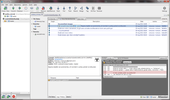
I was introduced to git a while ago, but somehow decided to go for Subversion. A few days ago a friend of mine pointed out SourceTree, a git GUI client for Windows and Mac. It’s not all GUI, all you die-hard CLI users are able to use their favorite tool. It hooks well with BitBucket, Stash, GitHub and Kiln. I opted for BitBucket, because it offers free private repositories.

The interface is, to my mind, very intuitive. You have a bookmark sidebar with your favorite projects, main window where most of the magic happens and of course the toolbar, where you can commit, checkout, remove, pull, push, branch, merge (and more) projects. For understanding git, Git Reference site can be helpful.

Once you create a new (local or remote) repository, the program will scan for any possible changes. Once a change has been detected, you will be able to commit them. In git lingo, this means that you will acknowledge these changes and apply them. SourceTree will keep a nice history tab for you, and you can revert to previous versions by simply “checking it out”. Once you’re happy with all the changes and you think your repo should see the light of day, you can Push it to your favorite git site, like BitBucket or GitHub. If you’re collaborating with others, you can always Fetch/Pull changes from the main site and have you repo up to date.

If you’re looking for version control, and you see yourself as a prospective (or current) collaborator, do give git and SourceTree a try.

SourceTree in action. Left is the bookmark sidebar and the main window is showing the history of my master branch. Click on image to enlarge (the image).

How to branch/fork a (StatET) project with SVN

I was introduced to version control at the 2011 Belgrade R+OSGeo in higher education summer school. I’ve been using it in my daily work ever since.

Recently the need to branch my project came up and this post describes how after a few hours of reading teh internets satisfied my need. In a nutshell, you should prepare your SVN repository to accept branches, branch your local project, dance. Yes, it’s as simple as that.

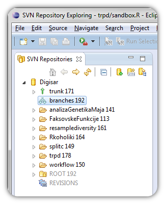
First, you need to prepare your repository to be able to accept branches. You do that by creating a “branches” directory. Probably the correct location is root of your SVN repository. At least that’s how it works for me.

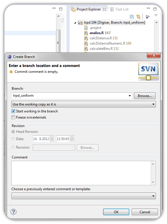
You now swith to StatET view and “branch” your project. Right-click your project, Team > Branch. Name your branch and check “Start working in the branch”.

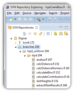
If you refresh your SVN repository, you should now see your branched project.

And if you checked the “Start working in this branch” your (local) project should automatically be looking at this branch.

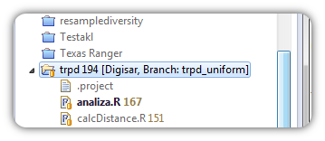
You’re ready to work on your branched/forked project. After you’re done, you can merge this branch with your original project. This aids in casual experimentation without long term consequences. Keep off of drugs, use protection, stay in school!

Show me yours and I’ll show you mine

I remember when I started with R, there was little processing power directed toward an IDE. I had enough problems with the syntax, loops and the like and R gui seemed adequate. When I started working on a heavy project, I had to knock it up a notch (bam!). After weeks of trial and error with various IDEs I settled for Eclipse. Year was 2010.
After two years, I feel very comfortable in my IDE of choice but I’ve always felt there’s some things I might be missing. That’s why I’m starting “show me yours and I’ll show you mine” project where I wish to collect workflow setup for working for programming and/or data analysis. The idea is to present your setup and comment on why you think it’s (in)efficient for you. I’ll start!

As mentioned, I use Eclipse with a plugin StatET. Eclipse (and StatET) depend on Java, so you’ll probably have to install either JDK or SDK. This may be a limiting factor for some. Eclipse offers a number of handy keyboard shortcuts (for instance CTRL+r+3 sends line/chunk to R, CTRL+r+s sources the entire file…), manages windows, provides different views and more.

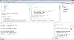
My setup has two code editing windows in the upper left corner, project explorer and task list (kudos to Andrie) on the right. Bottom half holds the R console and R help/tasks. I can easily navigate through files while debugging programs and handy keyboard shortcuts really cut down production time. I like having all windows handy. This is aided by Mylyn Task List plugin that helps you store and switch between individual sets of scripts. More about Mylyn can be found here. I also have a button to run knitr script which produces a pdf report (see previous post). I connect to a SVN server where I store my work. Switching to a SVN look is achieved by clicking the “SVN” icon in the top right corner.

I would encourage anyone interested in sharing their ideas about how to set up their workflow on this blog to send me a screenshot and a short description to my gmail account (romunov) or post about it on their own internet outlet (blog, personal website…) and send a traceback back here.

Getting knitr to work with StatET

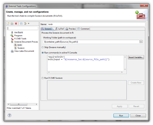
StatET (an Eclipse plug-in that can handle, among other things, R) offers support for writing Sweave (.Rnw) documents. This is done via the external tool dialog, where one creates a new “device” that takes in a document and runs it over appropriate functions and programs. In this case, Sweave and LaTeX. This dialog can, however, be modified to use function knit from package knitr. With a little luck, you can will be able to produce handsome looking pdfs with one click.

As I’ve already said, you will need to create your “knitr device”. You can reach the appropriate menu to external tools via Run > External tools > External tools configuration and create new “Sweave document processing” launch configuration. I have used the following options. Make sure you have package knitr installed.

 

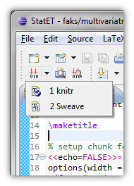
Assuming you have everything configured correctly, you can run the file through knitr with a single click*. You can do that by clicking the icon with three red arrows pointing at 010.

 

 

* Side note: You will probably need to put the documents you want to weave inside your workspace directory.

Write data (frame) to Excel file using R package xlsx

Writing to Excel files comes up rather often, especially if you’re collaborating with non-OSS users. There are several options, but I like the xlsx package way of doing things. Authors use Java to write to Excel files, which are basically compressed XML files.

Alright, let’s get cracking.

First, let’s create some data.

sample.dataframe

If you don’t have the file created yet, you can just write the data into a new file.

library(xlsx) #load the package
write.xlsx(x = sample.dataframe, file = "test.excelfile.xlsx",
        sheetName = "TestSheet", row.names = FALSE)

If you already have a file created, you can add data to a new sheet, or just add it to the existing one. Here’s how you would add a data.frame to columns D and E (result not shown).

workbook.sheets workbook.test addDataFrame(x = sample.dataframe, sheet = workbook.test,
   row.names = FALSE, startColumn = 4) # write data to sheet starting on line 1, column 4
saveWorkbook(workbook.sheets, "test.excelfile.xlsx") # and of course you need to save it.

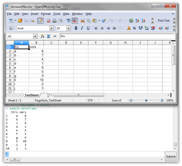
You can now open the file in your WYSIWYG editor.

Adding lines or points to an existing barplot

Sometimes you will need  to add some points to an existing barplot. You might try

par(mfrow = c(1,2))
df <- data.frame(stolpec1 = 10 * runif(10), stolpec2 = 30 * runif(10))
barplot(df$stolpec1)
lines(df$stolpec2/10) #implicitno x = 1:10
points(df$stolpec2/10) 

but you will get a funky looking line/points. It’s a bit squeezed. This happens because bars are not drawn at intervals 1:10, but rather on something else. This “else” can be seen if you save your barplot object. You will notice that it’s a matrix object with one column – these are values that are assumed on x axis. Now you need to feed this to your lines/points function as a value to x argument and you’re all set.

df.bar <- barplot(df$stolpec1)
lines(x = df.bar, y = df$stolpec2/10)
points(x = df.bar, y = df$stolpec2/10)

Another way of plotting this is using plotrix package. The controls are a bit different and it takes some time getting used to it.

library(plotrix)

barp(df$stolpec1, col = "grey70")
lines(df$stolpec2/10)
points(df$stolpec2/10)

 

Modeling sound pressure level of a rifle shot

Noise can be classified as pollution and lawmakers often (always?) treat it as such. Noise can have different origin points, point source being among the simplest to model. Because noise has broader health implications, being able to understand its propagation, a simple model can further our understanding in toning down or preventing excessive noise burden on the environment and its inhabitants. In this work, I will focus on firing range noise and the propagation of sound to the surrounding area.
Small scale firing ranges can be considered as point origin of noise. To make a simple predictive model, a number of assumptions and generalization are made. The reader should realize that this makes the model a bit less realistic.

When talking to experienced people, they will tell you that the distance between a firing range and the first house should be roughly 200 m. While there is no explicit mention of this number in Slovenian laws (yes, I’ve checked), there is a threshold of sound pressure level (SPL) of 75 dB. So, knowing the SPL of the rifle and we know the legal threshold, we can use a simple model to estimate approximate distance at which the SPL will fall to or below the aforementioned legal threshold.

A rifle shot produces a sound pressure level of about 170 dB, which is roughly the sound of a jet engine at a 30 m distance (see here).

Noise propagates and dissipates through the air with roughly (source)

p ~ 1/r

which gives us

L_2 = L_1 - 20 × log(r_2/r_1)

where

L_2 = sound level at  measured distance
L_1 = sound level at reference distance
r_1 = reference distance from source of the sound
r_2 = measured distance from the source

Using this model, we have accepted all sorts of assumptions, like calm weather, even terrain, even air pressure, no air resistance… Come to think of it, this model would be best suited for a desert in lovely weather. Nonetheless, it gives us a starting point.

I would be interested to hear from more knowledgeable readers on any potential mistakes and how to improve the model with regards to at least above assumptions.

Modeling this equation in R is trivial. Let’s write a function that will calculate L_2 for a sequence of r_2 values.

soundPressure <- function(r2, r1, L1) {
 L2 <- L1 - 20 * log(r1/r2)
 dL <- L1 - abs(L1 - L2) # this will give us the appropriate delta that we can use to plot our graph
 return(dL)
}

# let's define some parameters
distance <- seq(1, 1000, 1) # a vector of distances to be used as r_2
L1 <- 170
r1 <- 1

# this is the threshold level defined by the lawmaker
# we're actually interested in finding at what distance, the noise
# dissipates to this level
dB.level <- 75

# apply the above formula to every value in "distance"
dB <- sapply(distance, soundPressure, r1 = r1, L1 = L1)

# plotting
find.x <- which(round(dB) == dB.level)[1] # find which value is ~75 dB

plot(x = distance, y = dB, ylim = c(1, L1), xlab = "Distance (m)",
 ylab = "Sound pressure level (dB)", type = "l")
abline(h = dB.level, col = "red")
abline(v = find.x, col = "red")
# distance label
text(x = distance[find.x], y = 0, offset = 0.5, col = "black",
 pos = 4, labels = paste(distance[find.x], "m"), cex = 1.3)
# SPL
text(x = 0, y = dB.level, col = "black", labels = paste(dB.level, "dB"),
 cex = 1.3, offset = 1, pos = 1)

Result of the plotting is

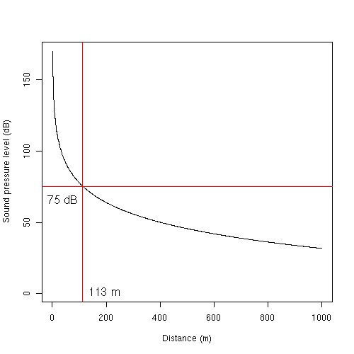
This tells us that the sound pressure level at roughly 113 m away from the rifle will be 75 dB (the legal threshold). Based on these results, a 200 m buffer around a firing range gives an estimate with a margin of around 100 m buffer.

As already mentioned, I would be happy to hear your comments on errors and how to improve the above model.

Dump R datasets into a single file

Should you need datasets that come with R and additional packages (you can access them via data()) in one single file, here’s what I did to dump the entire workspace into one file:

rm(list=ls())
data(list = data()$results[, 3])  # put datasets into your global environment
sink("datasets.txt")
for (i in 1:length(ls())) {
 cat("*****************", "\n")
 print(ls()[i])
 cat("*****************", "\n")
 print(get(ls()[i]))
 cat("\n")
}
sink()

This code can easily be adapted to dump individual dataset into its own file.

Bootstrap, strap-on, anal-yzing… statistics is getting weirder by the moment

I have spent the better portion of the day trying to get a bootstrap working. I have adapter a pre-written bootstrap function, but I wanted to use a generic function, mostly for reaping fame and glory. My hypothesis was that writing a hand-written, unoptimized function will consume more computer time than the generic, presumably optimized, boot() function. Was I wrong!

In this example, I random sample (with replacement) a vector of n values and store them in a matrix. These values that are written to the matrix are percent of values of our initial vector values that are smaller or equal to the bin number (see the code). Once we’ve got all the values, we can calculate the median by columns for further tinkering. There’s a lot of material covering bootstrapping on the Internet, but for a quick reference, see this Wikipedia entry. At this StackOverflow thread, Aniko provided me with valuable information on what I was doing wrong.

This is the code I used – first part is the hand written function, and the second part is my attempt at cracking the matter with a generic function.

require(Hmisc)

#generate fake data
data <- rchisq(500, df = 12)

#create bins
binx <- cut(data, breaks = 10)
binx <- levels(binx)
binx <- sub("^.*\\,", "", binx)
binx <- as.numeric(substr(binx, 1, nchar(binx) - 1))

#pre-allocate a matrix to be filled with samples
num.boots <- 10
output <- matrix(NA, nrow = num.boots, ncol = length(binx))

#do random sampling from the vector and calculate percent
#of values equal or smaller to the bin number (i)

for (i in 1:num.boots) {
 data.sample <- sample(data, size = length(data), replace = TRUE)
 data.cut <- cut(x = data.sample, breaks = 10)
 data.cut <- table(data.cut)/sum(table(data.cut))
 output[i, ] <- data.cut
}

#do some plotting
plot(1:10, seq(0, max(output), length.out = nrow(output)), type = "n", xlab = "", ylab = "")

for (i in 1:nrow(output)) {
 lines(1:10, output[i, 1:nrow(output)], lwd = "0.5")
}
output.median <- apply(output, 2, median)
output.sd <- apply(output, 2, sd)
sd.up <- output.median + output.sd * 1.96
sd.down <- output.median - output.sd * 1.96

lines(output.median, col="red", lwd = 3)
lines(sd.up, lty="dashed", col="green")
lines(sd.down, lty="dashed", col="green")
legend(x = 8, y = 0.25, legend = c("median", "0.95% CI"), col = c("red", "green"), lty = c("solid", "dashed"), lwd = c(3, 1))

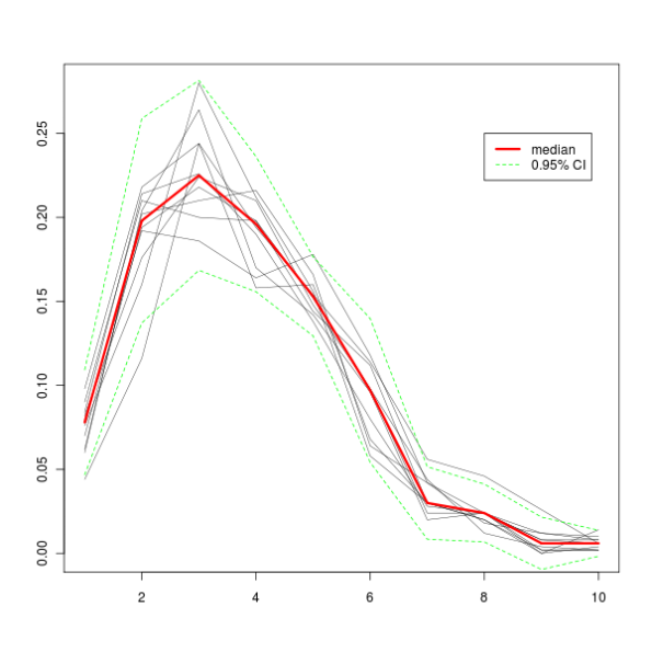
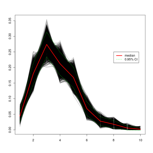
All this produces this graph.

Click to enlarge (the picture).

We can then try the power of the generic boot::boot() function that comes with the R core packages. The fun part of doing a bootstraping with the boot() function is to figure out how to write the statistic function correctly. If you look at the boot() help page (?boot) you will notice that you need to provide at least two parameters to the statistic argument: data and an index parameter. Help page says that the index parameter is a vector, which is a bit confusing from where I sit. In other words, this is actually a “an empty object” (let’s call the object i for now) that tells the boot() how to crawl over your data. If your data is in a form of a vector, you will place the index as you would use to subset a vector – object[i]. If it’s a data.frame and you want to re-sample rows, you would call object[i, ]… Let’s see a working example, things may be clearer there.

pairboot <- function(data, i, binx) {
 data.cut <- cut(x = data[i], breaks = 10)
 data.cut <- table(data.cut)/sum(table(data.cut))
 return(data.cut)
}

Notice the data[i] in the function. This will tell the boot() function to extract i elements of the data. If we had a data.frame, and rows were what we wanted to sample randomly, we would have written data[i, ].
And now we call the boot function to perform 10 “boots” on our data.

library(boot)
booty.call <- boot(data = data, statistic = pairboot, R = 10, binx = binx)

And here is the code to plot the output of the boot object (actually, it’s the print.boot object!). If you don’t believe me, try it on your own and see if you get a similar picture as above.

plot(1:10, seq(0, 1.5 * max(booty.call$t0), length.out = nrow(booty.call$t)), type = "n", xlab = "", ylab = "")
apply(booty.call$t, 1, function(x) lines(x, lwd = 0.5))
booty.call.median <- apply(booty.call$t, 2, median)
booty.call.sd <- apply(booty.call$t, 2, sd)
booty.call.sd.up <- booty.call.median + booty.call.sd * 1.96
booty.call.sd.down <- booty.call.median - booty.call.sd * 1.96
lines(booty.call.median, col="red", lwd = 3)
lines(booty.call.sd.up, lty="dashed", col="green")
lines(booty.call.sd.down, lty="dashed", col="green")
legend(x = 8, y = 0.25, legend = c("median", "0.95% CI"), col = c("red", "green"), lty = c("solid", "dashed"), lwd = c(3, 1))

The plot thickens!

Have I, by doing a bootstrap with a generic function, profited time-wise at all? Here are the elapse times for 10000 iterations for our hand written bootstrap function and the generic, respectively.

# user  system elapsed
#20.045   0.664  22.821

# user  system elapsed
#20.382   0.612  22.097

So you can see, I profit by 0.724 seconds. Was it worth it? 🙂 I can, for the moment, only wonder if I could improve the generic function to beat the hand-written one. Does anyone skilled in optimizing chip in any tips?

And here’s how a graph with 10000 iterations looks like. The green dashed lines represent a 95% confidence interval, which means that 95% of iterations fall between those two lines.

Bootstrap with 10000 iterations. CI is confidence interval.

How to calculate with dates and hours in R

A while ago I was asked whether calculating with datums and hours is possible in R. Especially, if you added an hours to 23:45 (say Jan 1, 2010) , would R know to jump to the next day – 00:45 (jan 2, 2010)? The answer is yes. Our only job is to tell R in what format our datum and time is. After we have done so, we can use these datums and times for different calculations.

Let’s say we have a vector (or any other object type) with datum and hour:

1.1.2010 11:35

We need to tell R that this is in fact a POSIX type object, whereas we need to specify which number corresponds to what. We will tell it that the first number is day, followed by a dot (.), followed by a month, followed by a dot… You get the picture. This is done through the format argument.

dtm <- strptime(c("1.1.2010 11:35"), format = "%d.%m.%Y %H:%M", tz = "CET")

While the inclusion of tz argument (time zone) is not applicable here, be careful if you’re calculating with datums and times from different time zones. For the following examples, I’ve added another element to the vector to spice things up.

> dtm
[1] "2010-01-01 11:35:00 CET" "2010-02-01 08:45:00 CET"
> str(dtm)
 POSIXlt[1:9], format: "2010-01-01 11:35:00" "2010-02-01 08:45:00"

For pedagogic purposes, I will make things a wee more complicated (at least for novice). Let’s write two simple (and I mean SIMPLE) yet not mandatory functions that will convert hours and minutes to seconds. Because calculating with POSIX objects is done via seconds (see below), by using these functions we free ourselves from typing 3 * 3600 every time we want to use 3 hours or 3*60 for 3 minutes. At least in my view, this makes the code (where we calculate) a bit more readable.

Here are the two functions:

hrs <- function(u) {
 x <- u * 3600
 return(x)
}

mns <- function(m) {
 x <- m * 60
 return(x)
}

This will add three hours to the current date/time values in dtm

> dtm + hrs(3)
[1] "2010-01-01 14:35:00 CET" "2010-02-01 11:45:00 CET"

This will add 3 hours and 10 minutes.

> dtm + hrs(3) + mns(10)
[1] "2010-01-01 14:45:00 CET" "2010-02-01 11:55:00 CET"

If we hadn’t used our functions, our input would look like this

> dtm + 3*3600 + 10*60
 [1] "2010-01-01 14:45:00 CET" "2010-02-01 11:55:00 CET"

See, I told you hrs() and mns() is more intuitive. 😛

We can also subtract. Let’s cut off 111 seconds

> dtm - 111
[1] "2010-01-01 11:33:09 CET" "2010-02-01 08:43:09 CET"

We are interested if datum will change if we add enough hours (or minutes). Let’s add 15 hours.

> dtm + hrs(15)
[1] "2010-01-02 02:35:00 CET" "2010-02-01 23:45:00 CET"

No surprises there – first element changed to the next day and the seconds element fell short for 15 minutes.

If we’re curious how far apart are two datums, we use the following function:

> difftime(dtm2[1], dtm2[2])
Time difference of -30.88194 days

All this and more can be also found in The R Book by Michael J. Crawley. This particular chapter can be accessed through the web. Data manipulations with R by Phil Specter can in part be previewed here (kudos to aL3xa for pointing it out). Help pages on datums and time classes can be found in

?DateTimeClasses